Introduction
There are many examples of how to use forecasting to save time and cost in a data science project, especially measuring simple or complex relationships among variables to accurately hit your target metrics over time and future-proof business decisions. For example, electric usage and solar power generation forecasting in the energy industry always helped businesses make the right calls in a competitive environment to save operating costs and, most importantly, the environment. Now, machine learning-driven forecasting and the availability of localized weather data are improving the accuracy of these predictions compared to the limitations of earlier statistical methods.
Note: Oracle Cloud Infrastructure Forecasting is currently in limited availability. To access Forecasting, goto Oracle Beta Programs page and click Oracle Data & AI Cloud Services Umbrella Beta Program.
In this blog, I will use the OCI forecasting service to demonstrate how to forecast solar energy generation with additional weather features. However, before we start the project, we need to understand that the efficacy of solar energy generation can be affected by various factors, including:
- Amount of sunlight: The amount of sunlight received at a particular location can affect the amount of solar energy panels produce.
- Panel orientation and tilt: The orientation and tilt of the solar panels can impact the amount of sunlight they receive and, therefore, their efficiency.
- Temperature: High temperatures can reduce the efficiency of solar panels, as they can cause the cells to overheat and produce less energy.
- Shading: Even partial solar panel shading can significantly reduce energy production, as shading can block incoming sunlight.
- Panel age and maintenance: The age and maintenance of solar panels can impact their efficiency, as older or poorly maintained solar panels may not perform as well as new, well-maintained ones.
- Weather conditions: Cloudy or rainy weather can significantly reduce the amount of sunlight reaching the solar panels, leading to decreased energy production.
Prepare your data
I collected the solar production data sample from a 10kw inverter with a data logger and 32 solar panels. The data logger collects data every 5min. Below is an example of the data collected:
| Date and time | Apparent power L1 feed-in point | PowerMeter | Apparent power L2 feed-in point | PowerMeter | Apparent power L3 feed-in point | PowerMeter | Effective power L1 feed-in point | PowerMeter | Effective power L2 feed-in point | PowerMeter | Effective power L3 feed-in point | PowerMeter | Voltage AC L1 feed-in point | PowerMeter | Voltage AC L2 feed-in point | PowerMeter | Voltage AC L3 feed-in point | PowerMeter | Apparent power | Symo 10.0-3-M (1) | Current AC L1 | Symo 10.0-3-M (1) | Current AC L2 | Symo 10.0-3-M (1) | Current AC L3 | Symo 10.0-3-M (1) | Current DC MPP1 | Symo 10.0-3-M (1) | Current DC MPP2 | Symo 10.0-3-M (1) | Energy | Symo 10.0-3-M (1) | Energy MPP1 | Symo 10.0-3-M (1) | Energy MPP2 | Symo 10.0-3-M (1) | Power factor | Symo 10.0-3-M (1) | Reactive power | Symo 10.0-3-M (1) | Specific yield | Symo 10.0-3-M (1) | Voltage AC L1 | Symo 10.0-3-M (1) | Voltage AC L2 | Symo 10.0-3-M (1) | Voltage AC L3 | Symo 10.0-3-M (1) | Voltage DC MPP1 | Symo 10.0-3-M (1) | Voltage DC MPP2 | Symo 10.0-3-M (1) | Consumed directly | Consumption | Energy from battery | Energy from grid | Energy to battery | Energy to grid | PV production |
|---|---|---|---|---|---|---|---|---|---|---|---|---|---|---|---|---|---|---|---|---|---|---|---|---|---|---|---|---|---|---|---|---|---|
| [dd.MM.yyyy HH:mm] |
[VA] |
[VA] |
[VA] |
[W] |
[W] |
[W] |
[V] |
[V] |
[V] |
[VA] |
[A] |
[A] |
[A] |
[A] |
[A] |
[Wh] |
[Wh] |
[Wh] |
[1] |
[VAr] |
[kWh/kWp] |
[V] |
[V] |
[V] |
[V] |
[V] |
[Wh] |
[Wh] |
[Wh] |
[Wh] |
[Wh] |
[Wh] |
[Wh] |
| 04.02.2021 00:00 |
297.26 |
229.49 |
952.11 |
108.31 |
86.41 |
697.73 |
249.02 |
248.7 |
245.46 |
0 |
0 |
0 |
0 |
0 |
0 |
0 |
0 |
0 |
0 |
0 |
0 |
0 |
0 |
0 |
5.3 |
3.8 |
0 |
74 |
0 |
74 |
0 |
0 |
0 |
| 04.02.2021 00:05 |
294.99 |
221.69 |
947.66 |
107.72 |
81.62 |
695.26 |
247.88 |
249.28 |
245.13 |
0 |
0 |
0 |
0 |
0 |
0 |
0 |
0 |
0 |
0 |
0 |
0 |
0 |
0 |
0 |
5.2 |
3.8 |
0 |
74 |
0 |
74 |
0 |
0 |
0 |
| 04.02.2021 00:10 |
302.28 |
206.37 |
949.57 |
107.74 |
132.51 |
687.95 |
248.07 |
249.19 |
245.62 |
0 |
0 |
0 |
0 |
0 |
0 |
0 |
0 |
0 |
0 |
0 |
0 |
0 |
0 |
0 |
5 |
3.7 |
0 |
77 |
0 |
77 |
0 |
0 |
0 |
| 04.02.2021 00:15 |
302.52 |
219.36 |
952.8 |
107.49 |
148.24 |
683.78 |
247.07 |
248.92 |
245.38 |
0 |
0 |
0 |
0 |
0 |
0 |
0 |
0 |
0 |
0 |
0 |
0 |
0 |
0 |
0 |
5.4 |
4 |
0 |
79 |
0 |
79 |
0 |
0 |
0 |
| 04.02.2021 00:20 |
293.45 |
198.22 |
945.72 |
107.5 |
110.21 |
689.39 |
247.29 |
248.54 |
245.61 |
0 |
0 |
0 |
0 |
0 |
0 |
0 |
0 |
0 |
0 |
0 |
0 |
0 |
0 |
0 |
5.5 |
3.9 |
0 |
75 |
0 |
75 |
0 |
0 |
0 |
| 04.02.2021 00:25 |
293.4 |
212.59 |
943.94 |
107.48 |
57.67 |
689.11 |
247.25 |
248.45 |
245.82 |
0 |
0 |
0 |
0 |
0 |
0 |
0 |
0 |
0 |
0 |
0 |
0 |
0 |
0 |
0 |
7.6 |
4.9 |
0 |
71 |
0 |
71 |
0 |
0 |
0 |
| 04.02.2021 00:30 |
293.98 |
222.36 |
943.2 |
107.52 |
82.78 |
688.91 |
247.54 |
248.98 |
245.52 |
0 |
0 |
0 |
0 |
0 |
0 |
0 |
0 |
0 |
0 |
0 |
0 |
0 |
0 |
0 |
7.3 |
4.7 |
0 |
74 |
0 |
74 |
0 |
0 |
0 |
| 04.02.2021 00:35 |
293.55 |
214.18 |
915.85 |
107.56 |
58.2 |
666.07 |
247.52 |
249.72 |
246.35 |
0 |
0 |
0 |
0 |
0 |
0 |
0 |
0 |
0 |
0 |
0 |
0 |
0 |
0 |
0 |
7.2 |
4.6 |
0 |
69 |
0 |
69 |
0 |
0 |
0 |
I collected the localized weather from the local weather station, and you can find your local weather station using the longitude and latitude of your solar panel location from weather.com. Once you have your location weather station id, you can retrieve hourly or daily weather data using your local station id using the weather.com API. Below is an example of the hourly weather data collected near my solar panels.
| stationID | tz | obsTimeUtc | obsTimeLocal | epoch | lat | lon | solarRadiationHigh | uvHigh | winddirAvg | humidityHigh | humidityLow | humidityAvg | qcStatus | metric.tempHigh | metric.tempLow | metric.tempAvg | metric.windspeedHigh | metric.windspeedLow | metric.windspeedAvg | metric.windgustHigh | metric.windgustLow | metric.windgustAvg | metric.dewptHigh | metric.dewptLow | metric.dewptAvg | metric.windchillHigh | metric.windchillLow | metric.windchillAvg | metric.heatindexHigh | metric.heatindexLow | metric.heatindexAvg | metric.pressureMax | metric.pressureMin | metric.pressureTrend | metric.precipRate | metric.precipTotal |
|---|---|---|---|---|---|---|---|---|---|---|---|---|---|---|---|---|---|---|---|---|---|---|---|---|---|---|---|---|---|---|---|---|---|---|---|---|
| ISYDNE991 | Australia/Sydney | 2021-02-03T13:04:58Z | 4/2/2021 0:04 | 1612357498 | -33.716 | 151.041 | 0 | 0 | 178 | 90 | 90 | 90 | 1 | 16.8 | 16.8 | 16.8 | 0 | 0 | 0 | 0 | 0 | 0 | 15.1 | 15.1 | 15.1 | 16.8 | 16.8 | 16.8 | 16.8 | 16.8 | 16.8 | 1001.12 | 1000.61 | 0 | 0 | 0 |
| ISYDNE991 | Australia/Sydney | 2021-02-03T13:09:46Z | 4/2/2021 0:09 | 1612357786 | -33.716 | 151.041 | 0 | 0 | 178 | 90 | 90 | 90 | 1 | 16.8 | 16.8 | 16.8 | 0 | 0 | 0 | 0 | 0 | 0 | 15.1 | 15.1 | 15.1 | 16.8 | 16.8 | 16.8 | 16.8 | 16.8 | 16.8 | 1000.91 | 1000.61 | 1.34 | 0 | 0 |
| ISYDNE991 | Australia/Sydney | 2021-02-03T13:14:50Z | 4/2/2021 0:14 | 1612358090 | -33.716 | 151.041 | 0 | 0 | 178 | 90 | 90 | 90 | 1 | 16.9 | 16.8 | 16.9 | 0 | 0 | 0 | 0 | 0 | 0 | 15.2 | 15.1 | 15.2 | 16.9 | 16.8 | 16.9 | 16.9 | 16.8 | 16.9 | 1001.12 | 1000.81 | 0 | 0 | 0 |
| ISYDNE991 | Australia/Sydney | 2021-02-03T13:19:54Z | 4/2/2021 0:19 | 1612358394 | -33.716 | 151.041 | 0 | 0 | 178 | 90 | 90 | 90 | 1 | 17 | 16.9 | 16.9 | 0 | 0 | 0 | 0 | 0 | 0 | 15.3 | 15.2 | 15.3 | 17 | 16.9 | 16.9 | 17 | 16.9 | 16.9 | 1001.02 | 1000.71 | -1.27 | 0 | 0 |
| ISYDNE991 | Australia/Sydney | 2021-02-03T13:24:58Z | 4/2/2021 0:24 | 1612358698 | -33.716 | 151.041 | 0 | 0 | 178 | 90 | 90 | 90 | 1 | 17.1 | 17 | 17.1 | 0 | 0 | 0 | 0 | 0 | 0 | 15.4 | 15.3 | 15.4 | 17.1 | 17 | 17.1 | 17.1 | 17 | 17.1 | 1001.02 | 1000.61 | 1.27 | 0 | 0 |
| ISYDNE991 | Australia/Sydney | 2021-02-03T13:29:46Z | 4/2/2021 0:29 | 1612358986 | -33.716 | 151.041 | 0 | 0 | 179 | 89 | 89 | 89 | 1 | 17.2 | 17.1 | 17.1 | 0 | 0 | 0 | 0 | 0 | 0 | 15.3 | 15.2 | 15.2 | 17.2 | 17.1 | 17.1 | 17.2 | 17.1 | 17.1 | 1000.91 | 1000.71 | -1.34 | 0 | 0 |
| ISYDNE991 | Australia/Sydney | 2021-02-03T13:34:50Z | 4/2/2021 0:34 | 1612359290 | -33.716 | 151.041 | 0 | 0 | 179 | 90 | 88 | 88.5 | 1 | 17.4 | 17.2 | 17.3 | 0 | 0 | 0 | 0 | 0 | 0 | 15.5 | 15.3 | 15.4 | 17.4 | 17.2 | 17.3 | 17.4 | 17.2 | 17.3 | 1000.81 | 1000.54 | -1.27 | 0 | 0 |
| ISYDNE991 | Australia/Sydney | 2021-02-03T13:39:54Z | 4/2/2021 0:39 | 1612359594 | -33.716 | 151.041 | 0 | 0 | 179 | 88 | 87 | 87.8 | 1 | 17.4 | 17.4 | 17.4 | 0 | 0 | 0 | 0 | 0 | 0 | 15.4 | 15.2 | 15.4 | 17.4 | 17.4 | 17.4 | 17.4 | 17.4 | 17.4 | 1000.81 | 1000.24 | -3.39 | 0 | 0 |
| ISYDNE991 | Australia/Sydney | 2021-02-03T13:44:58Z | 4/2/2021 0:44 | 1612359898 | -33.716 | 151.041 | 0 | 0 | 178 | 89 | 88 | 88.5 | 1 | 17.5 | 17.4 | 17.4 | 0 | 0 | 0 | 0 | 0 | 0 | 15.6 | 15.4 | 15.5 | 17.5 | 17.4 | 17.4 | 17.5 | 17.4 | 17.4 | 1000.71 | 1000.44 | 0 | 0 | 0 |
| ISYDNE991 | Australia/Sydney | 2021-02-03T13:49:46Z | 4/2/2021 0:49 | 1612360186 | -33.716 | 151.041 | 0 | 0 | 178 | 90 | 89 | 89.4 | 1 | 17.4 | 17.2 | 17.3 | 0 | 0 | 0 | 0 | 0 | 0 | 15.6 | 15.4 | 15.5 | 17.4 | 17.2 | 17.3 | 17.4 | 17.2 | 17.3 | 1000.61 | 1000.44 | 2.24 | 0 | 0 |
The above samples are the raw data that has to be processed and formatted to the data set that the OCI Forecasting service can process. I used a python script to consolidate the time series solar and weather data to the same time interval, in this case, hourly, and ensure the solar data has corresponding weather data using data/time. Below is an example:
Process weather data
data = pd.read_csv('hourly-weather-jan2022.csv',index_col=3,parse_dates=True)
temp = data.loc[:,['metric.tempHigh']]
groupByHour= temp.groupby([temp.index.month,temp.index.day, temp.index.hour]).mean()
groupByHour.index.set_names(["month", "day", "hour"], inplace=True)
groupByHour['ds'] = groupByHour.index.to_series().apply(lambda x: '2021-{0}-{1} {2}:00:00'.format(*x))
groupByHour['ds']= pd.to_datetime(groupByHour['ds'],format='%Y-%m-%d %H:%M:%S')
weatherData = pd.DataFrame(groupByHour.to_records())
weatherData.drop(['month', 'day', 'hour'], axis=1, inplace=True)
weatherData['metric.tempHigh']= weatherData['metric.tempHigh'].map('{:.2f}'.format)
weatherData.rename(columns = {'metric.tempHigh':'average_temp'}, inplace = True)
weatherData.rename(columns = {'ds':'solar_log_date'}, inplace = True)
weatherData['uid']="1"
weatherData.to_csv('processed-weather.csv', index=False)
Process solar production data
path =r'solarlogs'
all_files = glob.glob("../" + path + "/*.csv")
li = []
dateparse = lambda x: datetime.strptime(x, '%d.%m.%Y %H:%M')
date_cols = [0]
for filename in all_files:
    df = pd.read_csv(filename, parse_dates=date_cols, date_parser = dateparse, header=[0,1])
    df['DateTime']= pd.to_datetime(df.iloc[:, 0], yearfirst=True)
    li.append(df)
df = pd.concat(li)
n = df.shape[1]
print("Number of columns is:", n)
df.sort_values(by='DateTime', inplace=True)
columns_to_keep = [x for x in range(df.shape[1]) if x in [33,34]]
df = df.iloc[:, columns_to_keep]
df = df.fillna(0)
df.set_axis(['y', 'ds'], axis=1, inplace=True)
df.index =  df['ds']
df = df.groupby([df['ds'].dt.month, df['ds'].dt.day, df['ds'].dt.hour]).sum()
df.index.set_names(["month", "day", "hour"], inplace=True)
df['solar_log_date']= df.index.to_series().apply(lambda x: '2021-{0}-{1} {2}:00:00'.format(*x))
df['solar_log_date'] = pd.to_datetime(df['solar_log_date'],format='%Y-%m-%d %H:%M:%S')
df.rename(columns = {'y':'solar_production'}, inplace = True)
solar_data = df[(df['solar_log_date'] >= '2021-02-04') & (df['solar_log_date'] < '2021-02-11')]
solar_data=pd.DataFrame(solar_data.to_records())
solar_data.drop(['month', 'day', 'hour'], axis=1, inplace=True)
solar_data['solar_production']= solar_data['solar_production'].map('{:.2f}'.format)
solar_data['uid']="1"
solar_data.to_csv('processed-solar-log.csv', index=False)
Once the data is processed, you will have the primary and additional datasets to upload to the OCI Object Storage for the OCI Forecasting project. Primary and Additional Datasource columns should contain to 3 variables: a date, a time series Id, and a target variable. Below are the sample datasets:
Primary Dataset (Solar)
| solar_production | solar_log_date | uid |
|---|---|---|
| 0 | 2021-02-04 00:00:00 | 1 |
| 0 | 2021-02-04 01:00:00 | 1 |
| 0 | 2021-02-04 02:00:00 | 1 |
| 0 | 2021-02-04 03:00:00 | 1 |
| 0 | 2021-02-04 04:00:00 | 1 |
| 0 | 2021-02-04 05:00:00 | 1 |
| 73.37 | 2021-02-04 06:00:00 | 1 |
| 2872.53 | 2021-02-04 07:00:00 | 1 |
| 7088.68 | 2021-02-04 08:00:00 | 1 |
| 11621.51 | 2021-02-04 09:00:00 | 1 |
| 11382.73 | 2021-02-04 10:00:00 | 1 |
| 12226.46 | 2021-02-04 11:00:00 | 1 |
| 15723.57 | 2021-02-04 12:00:00 | 1 |
| 14089.95 | 2021-02-04 13:00:00 | 1 |
| 12867.34 | 2021-02-04 14:00:00 | 1 |
| 7998.88 | 2021-02-04 15:00:00 | 1 |
| 7024.32 | 2021-02-04 16:00:00 | 1 |
| 4530.79 | 2021-02-04 17:00:00 | 1 |
| 1531.83 | 2021-02-04 18:00:00 | 1 |
Additional Dataset (Weather)
| average_temp | solar_log_date | uid |
|---|---|---|
| 17.15 | 2021-02-04 00:00:00 | 1 |
| 16.63 | 2021-02-04 01:00:00 | 1 |
| 15.78 | 2021-02-04 02:00:00 | 1 |
| 15.31 | 2021-02-04 03:00:00 | 1 |
| 15.1 | 2021-02-04 04:00:00 | 1 |
| 14.82 | 2021-02-04 05:00:00 | 1 |
| 14.67 | 2021-02-04 06:00:00 | 1 |
| 16.28 | 2021-02-04 07:00:00 | 1 |
| 20.89 | 2021-02-04 08:00:00 | 1 |
| 22.66 | 2021-02-04 09:00:00 | 1 |
| 24.64 | 2021-02-04 10:00:00 | 1 |
| 26.37 | 2021-02-04 11:00:00 | 1 |
| 27.68 | 2021-02-04 12:00:00 | 1 |
| 28.56 | 2021-02-04 13:00:00 | 1 |
| 28.71 | 2021-02-04 14:00:00 | 1 |
| 28.53 | 2021-02-04 15:00:00 | 1 |
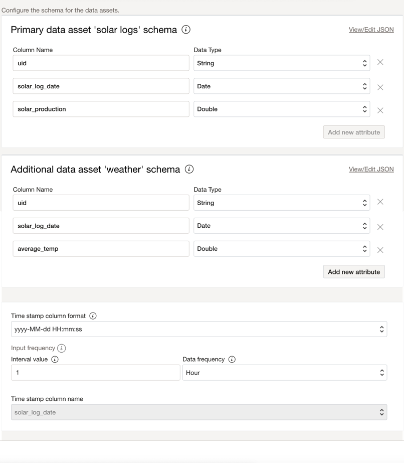
Using OCI Forecasting
Now, you can create a project and forecast using the datasets. Below is the configuration of my forecast project:
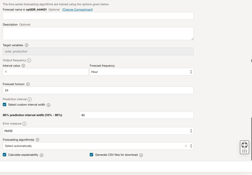
Error metrics compare a forecasting model’s data points with the actual historical data points and use them to measure errors for forecasting models. The forecasting service uses error metrics to compare the error in different models and chooses the best model that fits the actual values to predict future values. A list of supported error measures are:
- RMSE: RMSE stands for Root Mean Squared Error, a commonly used metric to evaluate the performance of a predictive model. It measures the square root of the average of the squared differences between the predicted and actual values. RMSE is often used in regression analysis to compare the accuracy of different models or assess a model’s performance on new data.
- MAPE: MAPE stands for Mean Absolute Percentage Error, a commonly used metric to evaluate the accuracy of a predictive model. It measures the average percentage difference between the predicted and actual values, dividing the absolute difference by the actual value. MAPE is often used in forecasting and demand planning to assess the accuracy of a model’s predictions, especially when dealing with data that has different scales or units.
- MSE: MSE stands for Mean Squared Error, a commonly used metric to evaluate the performance of a predictive model. It measures the average of the squared differences between the predicted and actual values. MSE is often used in regression analysis to compare the accuracy of different models or assess a model’s performance on new data. The smaller the MSE, the better the model makes accurate predictions.
- SMAPE: SMAPE stands for Symmetric Mean Absolute Percentage Error, a commonly used metric to evaluate the accuracy of a predictive model. It measures the average percentage difference between the predicted and actual values, where the absolute difference is divided by the sum of the predicted and actual values. Unlike MAPE, SMAPE is symmetric, which means it is not affected by the direction of the forecast error. SMAPE is often used in time series forecasting to compare the accuracy of different models or to assess the performance of a model on new data.
OCI Forecasting provides several algorithms. You can select more than one desired algorithm or let the service choose the algorithms automatically. Below is a list of supported algorithms:
Statistical Algorithms:
- NAIVE: Naïve
- SNAIVE: Seasonal Naïve
- SMA: Single Moving Average
- DMA: Double Moving Average
- HWSA: Holt – Winter’s Seasonal Additive
- HWSADAMPED: Holt – Winter’s Seasonal Additive method with a damped trend
- HWSM: Holt – Winter’s Seasonal Multiplicative
- HWSMDAMPED: Holt – Winter’s Seasonal Multiplicative method with a damped trend
- SES: Simple Exponential Smoothing
- DES: Double Exponential Smoothing
- DESDAMPED: Double Exponential Smoothing method with a damped trend
- SA: Seasonal Additive
- SM: Seasonal Multiplicative
- UAM: Ensemble Arithmetic Mean
- UHM: Ensemble Harmonic Mean
- ARIMA: Autoregressive Integrated Moving Average (ARIMA) Algorithm
Machine Learning Algorithms:
- PROPHET: Local Bayesian structural time series model from Prophet open source
- EFE: Endogenous Feature Engineering model
Deep Learning Algorithms:
- APOLLONET: A proprietary deep learning model
- PROBRNN: Probabilistic Recurrent Neural Network model
The calculate explainability option helps you understand the factors that influence the forecast, for each time series, for each time step of the forecast horizon, and remember to select the Generate CSV files for download option.
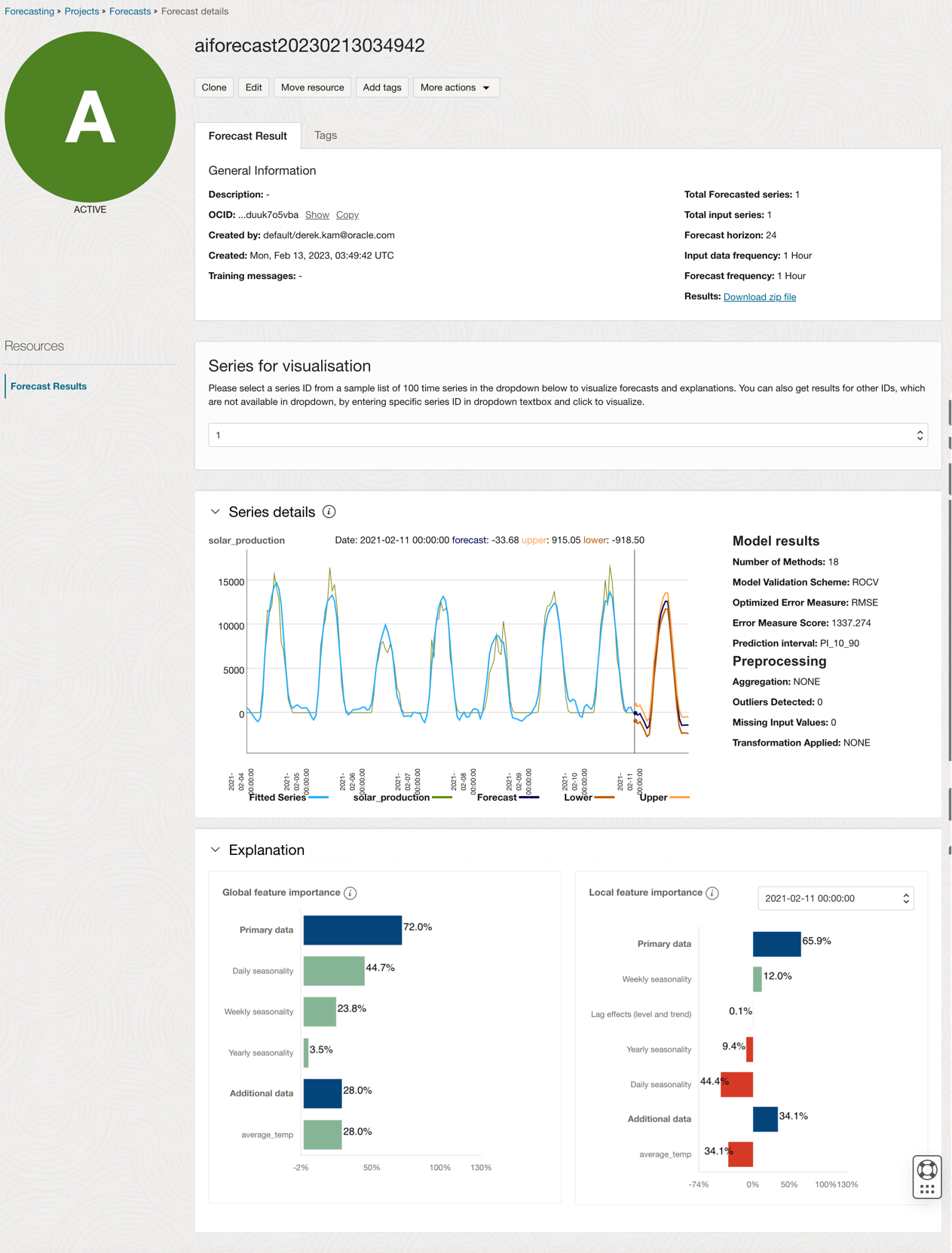
Forecast Results
Once the forecast is completed, it will create a zip file with the result to upload to another system or display on your dashboard. Below is the forecast result:
Below is the csv output:
Forecast report
| Series | bestModel | errorMeasureValue | errorMeasureName | numberOfMethodsFitted | seasonality | seasonalityMode | modelValidationScheme | preprocessingUsed.aggregation | preprocessingUsed.outlierDetected | preprocessingUsed.missingValuesImputed | preprocessingUsed.transformationApplied |
|---|---|---|---|---|---|---|---|---|---|---|---|
| 1 | prophet | 1337.273726 | RMSE | 18 | 24 | MULTIPLICATIVE | ROCV | NONE | 0 | 0 | NONE |
Forecast output
| Date | Series | input_value | fitted_value | forecast_value | p10 | p90 |
|---|---|---|---|---|---|---|
| 10/2/2021 15:00 | 1 | 11084.96 | 10626.8826 | |||
| 10/2/2021 16:00 | 1 | 6242.84 | 8111.57812 | |||
| 10/2/2021 17:00 | 1 | 4640.47 | 5031.19317 | |||
| 10/2/2021 18:00 | 1 | 1826.66 | 2702.22261 | |||
| 10/2/2021 19:00 | 1 | 363.86 | 845.741774 | |||
| 10/2/2021 20:00 | 1 | 0.04 | 115.922628 | |||
| 10/2/2021 21:00 | 1 | 0 | 577.757696 | |||
| 10/2/2021 22:00 | 1 | 0 | 633.438677 | |||
| 10/2/2021 23:00 | 1 | 0 | 0 | |||
| 11/2/2021 0:00 | 1 | -33.684476 | -918.49738 | 915.048155 | ||
| 11/2/2021 1:00 | 1 | -263.73133 | -1229.3797 | 688.025136 | ||
| 11/2/2021 2:00 | 1 | -102.16498 | -1023.5306 | 861.977084 | ||
| 11/2/2021 3:00 | 1 | -614.07374 | -1507.7627 | 307.978233 | ||
| 11/2/2021 4:00 | 1 | -1122.523 | -2059.0582 | -227.63318 | ||
| 11/2/2021 5:00 | 1 | -1753.3881 | -2688.378 | -926.50021 | ||
| 11/2/2021 6:00 | 1 | -1492.1362 | -2469.0342 | -575.77885 | ||
| 11/2/2021 7:00 | 1 | 944.145924 | 150.100499 | 1918.09045 | ||
| 11/2/2021 8:00 | 1 | 4772.80209 | 3769.66557 | 5698.56732 | ||
| 11/2/2021 9:00 | 1 | 7094.43269 | 6174.34066 | 7948.40642 | ||
| 11/2/2021 10:00 | 1 | 9768.72989 | 8849.60018 | 10667.3121 | ||
| 11/2/2021 11:00 | 1 | 11163.0014 | 10279.2137 | 11972.1156 | ||
| 11/2/2021 12:00 | 1 | 12045.671 | 11033.1883 | 13042.318 | ||
| 11/2/2021 13:00 | 1 | 12626.0861 | 11739.9175 | 13599.8574 | ||
| 11/2/2021 14:00 | 1 | 12622.2105 | 11741.7464 | 13565.0243 | ||
| 11/2/2021 15:00 | 1 | 10334.6912 | 9357.70722 | 11153.7107 | ||
| 11/2/2021 16:00 | 1 | 7307.00861 | 6403.09643 | 8227.05439 | ||
| 11/2/2021 17:00 | 1 | 4397.1661 | 3377.09405 | 5266.27713 | ||
| 11/2/2021 18:00 | 1 | 1356.04439 | 369.286183 | 2194.5948 | ||
| 11/2/2021 19:00 | 1 | -633.14913 | -1578.995 | 287.310187 | ||
| 11/2/2021 20:00 | 1 | -1421.4896 | -2316.7956 | -474.3533 | ||
| 11/2/2021 21:00 | 1 | -1412.6998 | -2286.0555 | -514.41326 | ||
| 11/2/2021 22:00 | 1 | -1378.8391 | -2292.3135 | -433.92763 | ||
| 11/2/2021 23:00 | 1 | -1420.7344 | -2367.9554 | -497.93322 |
Conclusion
A few takeaways from my experience in forecasting solar energy production using OCI Forecasting Service:
- The accuracy of weather forecasts can vary depending on several factors, such as the lead time of the forecast, the location, the weather conditions, and the forecasting methods used. Generally, short-term weather forecasts (up to 3 days) are more accurate than long-term forecasts (beyond 7 days). The accuracy of weather forecasts can also depend on the specific location, as some areas may have more complex weather patterns or fewer monitoring stations. For this use case, I only use the average hourly temperature.
- Add other features/factors as additional data from your solar inverter data that might affect solar energy production, like the age of the solar panel and inverter.
- For this use case, only forecast using a maximum of 7 days of weather data.
- When creating the forecast project using the data asset, remember the timestamp or date column’s data type shall be a date, the time-series name data type shall be string, and the target column data type shall be double or int.
- Let the service choose the algorithms automatically but experiment on different error metrics to compare a forecasting model.
- Create an architecture to automatically ingest the data from the Object Storage using OCI Events and process in OCI Functions or OCI Data Integration before running the OCI Forecasting Service. Here is the link to the reference architecture: Use OCI Forecasting to quickly create forecasts for your business
- Remember to name your data asset when you create a forecast in OCI Forecasting; otherwise, it is hard to find the data asset to use for other forecasts or projects. If you forgot to name it when you created it, you could always go back to rename it later.
- Forecasting has an upper limit for each file: 100,000 time-series items with 1,500 data points per series. Forecasting has no lower limit for the number of time-series items. For this use case, I have only one time-series item and use the 7 days hourly data, but if you use a 5min interval or lower data point, you exceed the allowed data point limit.
- Ensure the length of the additional data series is greater than or equal to the size of the primary series plus the forecast horizon. That means you must provide future values for the prediction timestamps. For example, to forecast the next two weeks’ solar production, provide values for the next two weeks. Also, Missing values are not allowed in the additional data, and the dates must match the primary dataset.
- As you cannot set the floor and cap forecast values, you might need to process the forecast result data before you display it on your dashboard. In this use case, the forecast value for solar generation cannot be negative. Also, it should be at most 10kw as the inverter’s maximum capacity is 10kw.